Show setup information.

knitr::opts_chunk$set(collapse = TRUE)
pacman::p_load(kableExtra, DT, htmlwidgets, htmltools, magick, 
               install = FALSE, update = FALSE)

Data Availability

All files generated in this workflow can be downloaded from figshare.

File names and descriptions:

cc-kraken.html: Short-read Kraken Krona plots for site Coral Caye (cc).
cr-kraken.html: Short-read Kraken Krona plots for site Cayo Roldan Caye (cr).
water_kaiju_mar.html: Contig Kaiju Krona plots against the mar database.
water_kaiju_nr.html: Contig Kaiju Krona plots against the nr database.

QC & Contig Stats

QC Results

The first thing we should do is look at the results of the initial QC step. For each sample, anvi’o spits out individual quality control reports. Thankfully anvi’o also concatenates those files into one table. This table contains information like the number of pairs analyzed, the total pairs passed, etc.

Assembly Results

Next we can look at the results of the co-assembly, the number of HMM hits, and the estimated number of genomes. These data not only give us a general idea of assembly quality but will also help us decide parameters for automatic clustering down the road.

We can use anvi’o to generate a simple table of contig stats for this assembly.

anvi-display-contigs-stats 03_CONTIGS/WATER-contigs.db -o 03_CONTIGS/WATER-contig-stats -o contig-stats.txt

You can download a text version of the table using the table buttons.

Krona Plots Explained

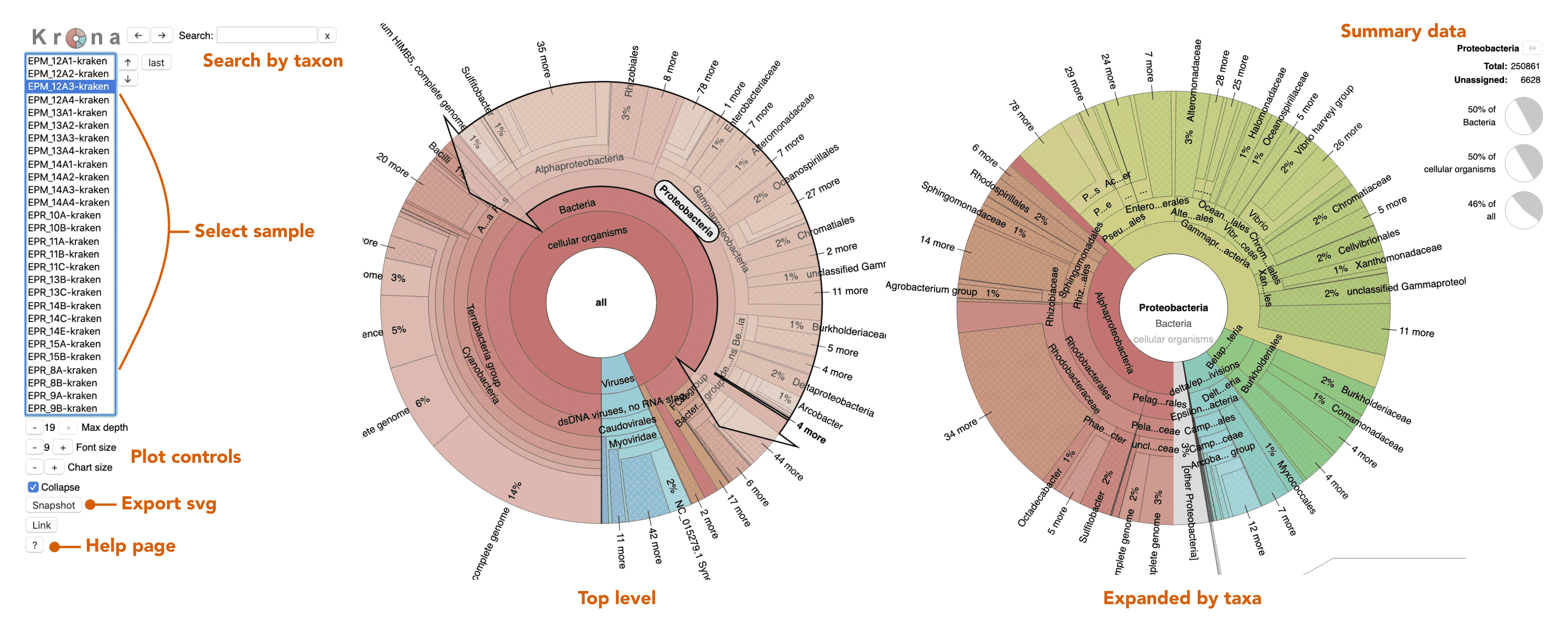
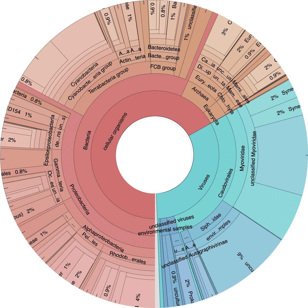
Next let’s take a look at the taxonomic breakdown from the KrakenUniq classification of short reads. There is a lot of data here, so we decided to present these as standalone HTML pages that contain separate Krona (Ondov, Bergman, and Phillippy 2011) plots for each sample. In brief, a Krona plot allow hierarchical data to be explored with multi-layered pie charts. These charts are interactive. We will use these on a few occasions, so it is worth explaining in a little more detail.

Below is an example of a Kraken taxonomy plot. The plot on the left is the top level view and the plot on the right is the expanded view. Inner rings represent higher taxonomic ranks.

For example, the two most inner rings are cellular organisms and viruses. Taxonomic ranks decrease towards the outside. When a group is expanded the inner ring becomes the highest rank. For example, in the plot of the right we expanded the Proteobacteria (which is a phylum) so the classes form the inner rings.

**Example of a Krona plot**. The **left panel** controls aspects of the plot. Search by taxon name, select a specific sample, control font size, etc. If you were to click once over a taxa on the left plot, the group is highlighted. Double-click to expand the group as seen on the right. Upper right corner provides a summary of the expanded group.

Short-read Taxonomy

Since the Kraken classification was performed BEFORE the assembly we can look at the Krona plots for each individual sample. Here samples are separated by site.

CAYO ROLDAN
Hypoxic & Normoxic

CRAWL CAYE
Normoxic

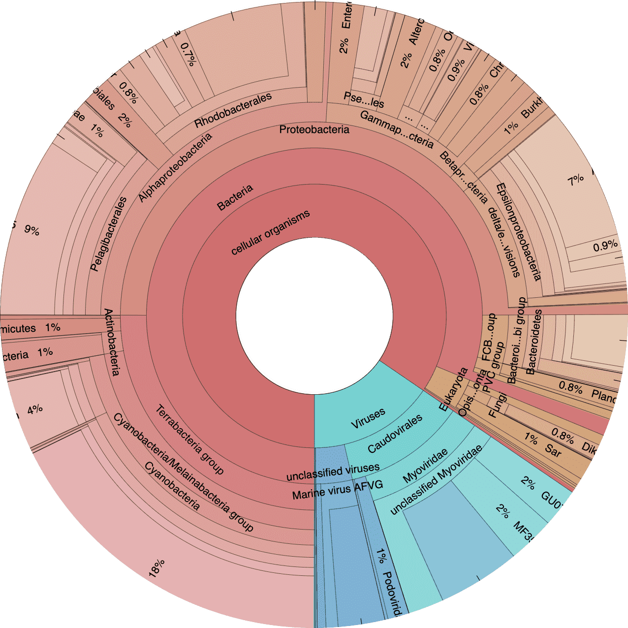
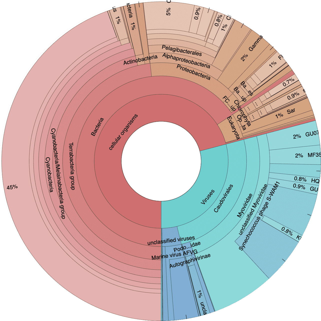
Click on an image to explore the diversity plots.

Since these plots are web hosted, I decided to keep only the first 10 ranks from the classification files to make the files smaller*. To do this we can use the following command, which pulls out only the ranks we are interested in.

cut -f 1-10 WROL_1914-kraken.krona > WROL_1914-kraken-TRIM.krona

If we want to create a taxonomic summary table for the samples we can easily do that in anvio by accessing the layer_additional_data table from the merged profile database.

anvi-export-table 06_MERGED/WATER/PROFILE.db --table layer_additional_data -o water-layer_additional_data.txt

And then we simply parse out the class data and make a table.

You can download a text version of the table using the table buttons.

Mapping Results

Let’s go ahead and look at the mapping results. This took a little swindling but in the end this crude approach worked. First we needed all the bowtie.log files from the 00_LOGS directory and grab the first line of each file, which has the total number of individual reads that were paired (after QC) in each sample.

Just like we did above, we needed to grab the layer_additional_data from the merged profile databases. This table contains total_reads_mapped, num_SNVs_reported, and the taxonomic info from the short-read Kraken annotations.

anvi-export-table 06_MERGED/WATER/PROFILE.db --table layer_additional_data -o water-layer_additional_data.txt

What we want is a table with sample, total_reads, total_reads_mapped, and num_SNVs_reported. After a little fancy grep work in BBEdit (the free mode) we have a table the looks like this…

You can download a text version of the table using the table buttons.

Contig Classification

Now we move on to the classification of contigs from the assembly. This means that we cannot look at individual samples because we co-assembled all of the data. We start with the Kaiju classification, again using the Krona plots. Remember we classified the contigs against both the nr and mar databases. Use the panels below to access the classifications for the assembly.

Kaiju classification
mar database

Kaiju classification
nr database

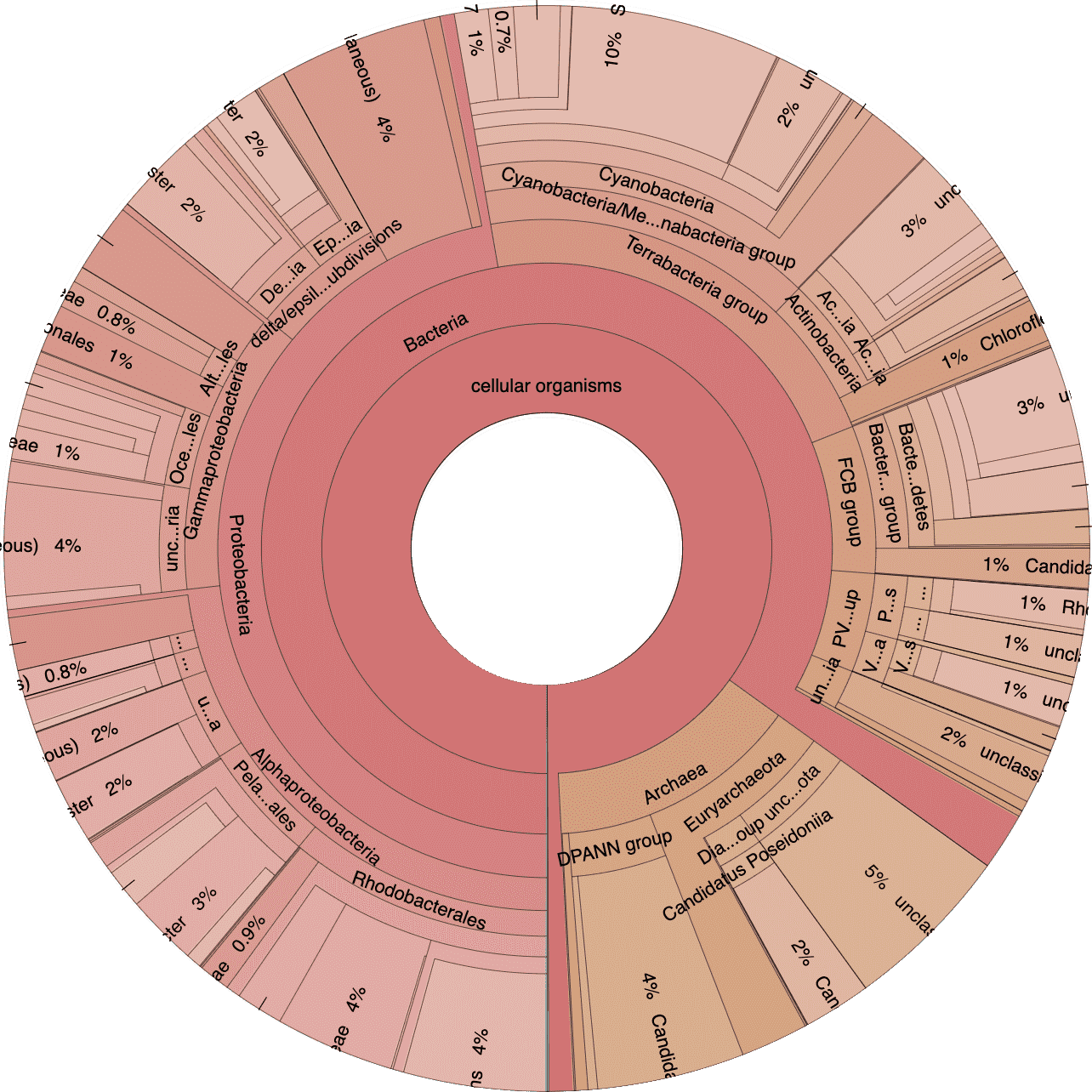
Click on an image to explore the diversity plots.

We will get into much more of the annotation data later, including the various functional annotations. For now though we have a pretty good idea of the shape and nature of these datasets.

Source Code

The source code for this page can be accessed on GitHub by clicking this link.