Show setup information.
knitr::opts_chunk$set(collapse = TRUE)
pacman::p_load(kableExtra, DT, htmlwidgets, htmltools,
               DiagrammeR, DiagrammeRsvg, rsvg, readr,
               tidyverse, plyr, data.table,
               install = FALSE, update = FALSE)
Data Availability
All files generated in this workflow can be downloaded from figshare.
File names and descriptions:
- 01_MAG04_PAN Pangenomic analysis of MAG04.
- 02_MAG04_PHYLOGENOMICS Phylogenomic analysis of MAG04. You can use the anvi’o commands described in the workflow to visualize the data.
What we want to do here is compare MAG041 to publicly available genomes. We will generally follow workflow similar to the one presented for MAG02.
anvi-estimate-scg-taxonomy -c 18_NR-MAGs-SPLIT/WATER_MAG_00004/CONTIGS.db| MAG | total_scgs | supporting_scgs | taxonomy |
|---|---|---|---|
| WATER_MAG_00004 | 18 | 13 | Bacteria / Proteobacteria / Alphaproteobacteria / Rhodobacterales / Rhodobacteraceae / Aliiroseovarius / Aliiroseovarius sp004360145 |
Getting Genomes from NCBI
For this workflow we largely follow the tutorial on Accessing and including NCBI genomes in ’omics analyses in anvi’o by Alon Shaiber and Meren.
We need genomes to compare to our MAG. As the tutorial explains, we can either use the taxa name itself or the TaxID. But before that we need to get the gimme_taxa.py helper script by by Joe R. J. Healey that allows us to download genomes from NCBI. Slick.
wget https://raw.githubusercontent.com/kblin/ncbi-genome-download/master/contrib/gimme_taxa.pyWe can start with the taxa names themselves.
Getting TaxIDs to Download
python gimme_taxa.py Aliiroseovarius \
                     -o Aliiroseovarius-for-ngd.txt
We 24 hits for Aliiroseovarius.
What about the TaxID?
We need to head to NCBI’s Taxonomy Browser and get the parent TaxID by searching for the taxon name of interest, in this case Aliiroseovarius.
Aliiroseovarius is TaxID 1658781. We can also see from the file Aliiroseovarius-for-ngd.txt that the parent TaxID of Aliiroseovarius is 1658781. Nice.
python gimme_taxa.py 1658781 \
                     -o Aliiroseovarius-TaxIDs-for-ngd.txt
Again, we get 24 hits. The results of using TaxID and taxon name were identical, however that is not always the case, so it is good to check.
Since we only need the TaxIDs, we can rerun the command like so:
python gimme_taxa.py 1658781 \
                     -o Aliiroseovarius_Group-TaxIDs-for-ngd-just-IDs.txt \
                     --just-taxids
As the command implies, we only get a list of TaxIDs. Moving on,
Downloading Genomes from NCBI
To download genomes using the TaxIDs, we need a collection of scripts called ncbi-genome-download. See the GitHub repo for installation instructions. We have a choice of where to look for genomes using the -s flag—either Genbank or Refseq
ncbi-genome-download -t Aliiroseovarius_Group-TaxIDs-for-ngd-just-IDs.txt \
                      bacteria \
                      -o 00_Aliiroseovarius_Genbank \
                      --metadata Aliiroseovarius-NCBI-METADATA.txt \
                      -s genbank
We tested both options and found that the -s genbank returned 28 genomes and -s refseq returned 24. We compared the two lists and found nothing unique in the Refseq database so we will continue with the GenBank set.
Processing NCBI Genomes
A metadata file is also created by ncbi-genome-download.
column -t Aliiroseovarius-NCBI-METADATA.txt | head -n 4assembly_accession bioproject biosample wgs_master excluded_from_refseq refseq_category relation_to_type_material taxid species_taxid organism_name infraspecific_name isolate version_status assembly_level release_type genome_rep seq_rel_date asm_name submitter gbrs_paired_asm paired_asm_comp ftp_path local_filename
GCA_001307765.1 PRJNA291771 SAMN03952659 LKBA00000000.1 representative genome assembly from type material 154981 154981 Aliiroseovarius crassostreae strain=CV919-312 latest Contig Major Full 2015/10/07 ASM130776v1 University of Rhode Island GCF_001307765.1 identical ftp://ftp.ncbi.nlm.nih.gov/genomes/all/GCA/001/307/765/GCA_001307765.1_ASM130776v1 ./00_Aliiroseovarius_Genbank/genbank/bacteria/GCA_001307765.1/GCA_001307765.1_ASM130776v1_genomic.gbff.gz
GCA_900116725.1 PRJEB17594 SAMN04488527 FPBS00000000.1 na assembly from type material 154981 154981 Aliiroseovarius crassostreae strain=DSM 16950 latest Scaffold Major Full 2016/11/02 IMG-taxon 2619619030 annotated assembly DOE - JOINT GENOME INSTITUTE GCF_900116725.1 identical ftp://ftp.ncbi.nlm.nih.gov/genomes/all/GCA/900/116/725/GCA_900116725.1_IMG-taxon_2619619030_annotated_assembly ./00_Aliiroseovarius_Genbank/genbank/bacteria/GCA_900116725.1/GCA_900116725.1_IMG-taxon_2619619030_annotated_assembly_genomic.gbff.gz
GCA_007004645.1 PRJNA548260 SAMN12012166 VICH00000000.1 representative genome assembly from type material 985055 985055 Aliiroseovarius halocynthiae strain=MA1-10 latest Scaffold Major Full 2019/07/15 ASM700464v1 Xinxiang Medical University GCF_007004645.1 identical ftp://ftp.ncbi.nlm.nih.gov/genomes/all/GCA/007/004/645/GCA_007004645.1_ASM700464v1 ./00_Aliiroseovarius_Genbank/genbank/bacteria/GCA_007004645.1/GCA_007004645.1_ASM700464v1_genomic.gbff.gzAnvi’o has a script that takes this metadata file and generates a fasta.txt file in the format compatible with anvi’o workflows. We will use the --exclude-gene-calls-from-fasta-txt because we want to do our own gene calling.
anvi-script-process-genbank-metadata -m Aliiroseovarius-NCBI-METADATA.txt \
                                     -o 01_Aliiroseovarius-NCBI-GENOMES \
                                     --output-fasta-txt Aliiroseovarius-fasta.txt \
                                     --exclude-gene-calls-from-fasta-txt
This command returns a directory, 01_Aliiroseovarius-NCBI-GENOMES full of fasta files and the file Aliiroseovarius-fasta.txt, which contains the name and fasta file path for each genome.
name    path
Aliiroseovarius_crassostreae_GCA_001307765_1    /pool/genomics/stri_istmobiome/data/TEMP/Aliiroseovarius/ALIIROSEOVARIUS/Aliiroseovarius-NCBI-GENOMES/Aliiroseovarius_crassostreae_GCA_001307765_1-contigs.fa
Aliiroseovarius_marinus_GCA_004360145_1 /pool/genomics/stri_istmobiome/data/TEMP/Aliiroseovarius/ALIIROSEOVARIUS/Aliiroseovarius-NCBI-GENOMES/Aliiroseovarius_marinus_GCA_004360145_1-contigs.fa
Aliiroseovarius_halocynthiae_GCA_007004645_1    /pool/genomics/stri_istmobiome/data/TEMP/Aliiroseovarius/ALIIROSEOVARIUS/Aliiroseovarius-NCBI-GENOMES/Aliiroseovarius_halocynthiae_GCA_007004645_1-contigs.fa
We need to add our MAG to the fasta directory and its name to the Aliiroseovarius-fasta.txt file. We will also change the names produced by anvi-script-process-genbank-metadata since they are not very meaningful. We can use the Aliiroseovarius-NCBI-METADATA.txt file, specifically the organism_name, infraspecific_name, and/or isolate columns to cobble together new genome names. I wish I could say I had a clever way to do this task, but really it was just some copying and pasting.
If you change the names they MUST be unique and contain no spaces, periods, dashes, or other weird characters. Letters, numbers, and underscores only.
Running Snakemake Contigs Workflow
Now it is time for some comparisons. First we will run the contigs workflow since this will produce annotated contig databases and properly formatted fasta files for all genomes. We will need these for phylogenomics. Ok, renamed file in hand, we use Snakemake workflow (Köster and Rahmann 2012) to run the built-in anvi’o contigs workflow. If you do not know what workflows are available you can run this command:
anvi-run-workflow --list-workflowsWARNING
===============================================
If you publish results from this workflow, please do not forget to cite
snakemake (doi:10.1093/bioinformatics/bts480)
Available workflows ..........................: contigs, metagenomics, pangenomics, phylogenomicsNext, we need a config file for the contigs workflow. This file tells anvi’o what commands to run and how to run them. We run this command to generate a default config file, which can be modified as you see fit. Some commands we chose not to run but they remain in the workflow for posterity.
anvi-run-workflow -w contigs --get-default-config contigs-default-config.jsonShow/hide JSON-formatted configuration file.
{
    "fasta_txt": "Aliiroseovarius-fasta-rename.txt",
    "anvi_gen_contigs_database": {
        "--project-name": "{group}",
        "--description": "",
        "--skip-gene-calling": "",
        "--ignore-internal-stop-codons": "",
        "--skip-mindful-splitting": "",
        "--contigs-fasta": "",
        "--split-length": "",
        "--kmer-size": "",
        "--skip-predict-frame": "",
        "--prodigal-translation-table": "",
        "threads": ""
    },
    "centrifuge": {
        "threads": 2,
        "run": "",
        "db": ""
    },
    "anvi_run_hmms": {
        "run": true,
        "threads": 20,
        "--installed-hmm-profile": "",
        "--hmm-profile-dir": "",
        "--also-scan-trnas": ""
    },
    "anvi_run_kegg_kofams": {
        "run": true,
        "threads": 20,
        "--kegg-data-dir": "/pool/genomics/stri_istmobiome/dbs/kegg_kofam/",
        "--hmmer-program": "",
        "--keep-all-hits": "",
        "--log-bitscores": "",
        "--just-do-it": ""
    },
    "anvi_run_ncbi_cogs": {
        "run": true,
        "threads": 20,
        "--cog-data-dir": "/pool/genomics/stri_istmobiome/dbs/cog_db/",
        "--sensitive": "",
        "--temporary-dir-path": "/pool/genomics/stri_istmobiome/dbs/cog_db/tmp/",
        "--search-with": ""
    },
    "anvi_run_scg_taxonomy": {
        "run": true,
        "threads": 20,
        "--scgs-taxonomy-data-dir": ""
    },
    "anvi_run_trna_scan": {
        "run": true,
        "threads": 20,
        "--trna-cutoff-score": ""
    },
    "anvi_script_reformat_fasta": {
        "run": true,
        "--prefix": "{group}",
        "--simplify-names": true,
        "--keep-ids": "",
        "--exclude-ids": "",
        "--min-len": "",
        "--seq-type": "",
        "threads": ""
    },
    "emapper": {
        "--database": "bact",
        "--usemem": true,
        "--override": true,
        "path_to_emapper_dir": "",
        "threads": ""
    },
    "anvi_script_run_eggnog_mapper": {
        "--use-version": "0.12.6",
        "run": "",
        "--cog-data-dir": "",
        "--drop-previous-annotations": "",
        "threads": ""
    },
    "gen_external_genome_file": {
        "threads": ""
    },
    "export_gene_calls_for_centrifuge": {
        "threads": ""
    },
    "anvi_import_taxonomy_for_genes": {
        "threads": ""
    },
    "annotate_contigs_database": {
        "threads": ""
    },
    "anvi_get_sequences_for_gene_calls": {
        "threads": ""
    },
    "gunzip_fasta": {
        "threads": ""
    },
    "reformat_external_gene_calls_table": {
        "threads": ""
    },
    "reformat_external_functions": {
        "threads": ""
    },
    "import_external_functions": {
        "threads": ""
    },
    "anvi_run_pfams": {
        "run": true,
        "--pfam-data-dir": "/pool/genomics/stri_istmobiome/dbs/pfam_db/",
        "threads": 20
    },
    "output_dirs": {
        "FASTA_DIR": "02_FASTA",
        "CONTIGS_DIR": "03_CONTIGS",
        "LOGS_DIR": "00_LOGS"
    },
    "max_threads": "",
    "config_version": "2",
    "workflow_name": "contigs"
}
We can also run a couple of sanity checks to make sure everything is good before starting the job. How about a workflow graph to visually inspect the steps?
anvi-run-workflow -w contigs -c contigs-default-config.json --save-workflow-graphWARNING
===============================================
If you publish results from this workflow, please do not forget to cite
snakemake (doi:10.1093/bioinformatics/bts480)
WARNING
===============================================
We are initiating parameters for the contigs workflow
WARNING
===============================================
You chose to define --temporary-dir-path for the rule anvi_run_ncbi_cogs in the
config file as /pool/genomics/stri_istmobiome/dbs/cog_db/tmp/. while this is
allowed, know that you are doing so at your own risk. The reason this is risky
is because this rule uses a wildcard/wildcards and hence is probably running
more than once, and this might cause a problem. In case you wanted to know,
these are the wildcards used by this rule: {group}
Workflow DOT file ............................: workflow.dot
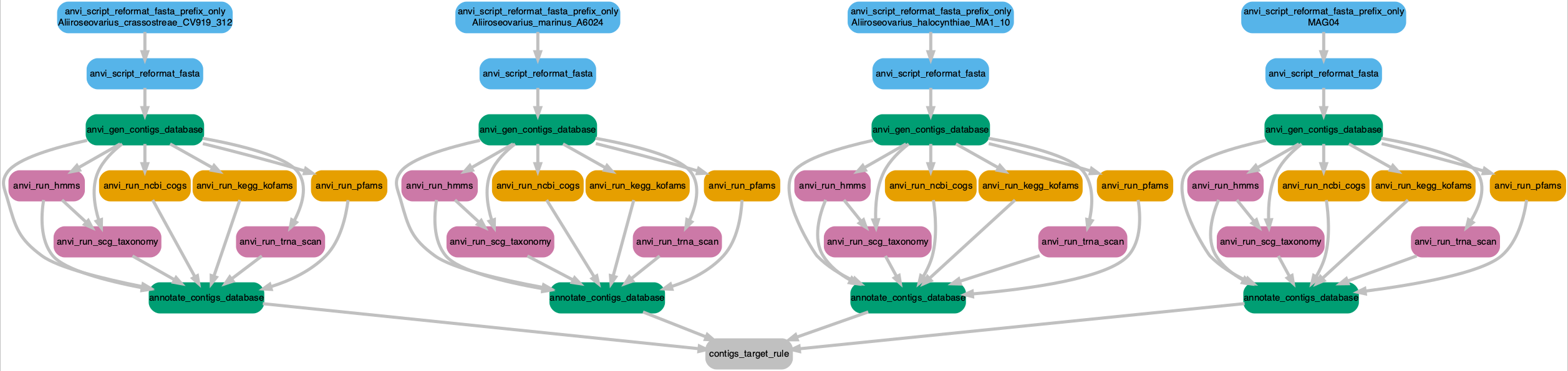
Workflow PNG file ............................: workflow.pngSuccess. Let’s have a look at the workflow. Only four genomes are shown for clarity but each step will be conducted for all genomes.
Click on the image to zoom in or download a copy.
Show/hide DAG R Code script
````
```{r workflow2, eval=FALSE}
dag <- grViz ("
digraph boxes_and_circles {
  graph [layout = dot, align=center]

  node [shape = rectangle, style = 'rounded,filled' fontname=sans, fontsize=12, penwidth=4]
  edge[penwidth=4, color=grey];


0[label = 'contigs_target_rule', color = 'grey'];
1[label = 'annotate_contigs_database', color = '#009E73'];
2[label = 'annotate_contigs_database', color = '#009E73'];
3[label = 'annotate_contigs_database', color = '#009E73'];
4[label = 'annotate_contigs_database', color = '#009E73'];
5[label = 'anvi_gen_contigs_database', color = '#009E73'];
6[label = 'anvi_run_hmms', color = '#CC79A7'];
7[label = 'anvi_run_ncbi_cogs', color = '#E69F00'];
8[label = 'anvi_run_kegg_kofams', color = '#E69F00'];
9[label = 'anvi_run_scg_taxonomy', color = '#CC79A7'];
10[label = 'anvi_run_trna_scan', color = '#CC79A7'];
11[label = 'anvi_run_pfams', color = '#E69F00'];
12[label = 'anvi_gen_contigs_database', color = '#009E73'];
13[label = 'anvi_run_hmms', color = '#CC79A7'];
14[label = 'anvi_run_ncbi_cogs', color = '#E69F00'];
15[label = 'anvi_run_kegg_kofams', color = '#E69F00'];
16[label = 'anvi_run_scg_taxonomy', color = '#CC79A7'];
17[label = 'anvi_run_trna_scan', color = '#CC79A7'];
18[label = 'anvi_run_pfams', color = '#E69F00'];
19[label = 'anvi_gen_contigs_database', color = '#009E73'];
20[label = 'anvi_run_hmms', color = '#CC79A7'];
21[label = 'anvi_run_ncbi_cogs', color = '#E69F00'];
22[label = 'anvi_run_kegg_kofams', color = '#E69F00'];
23[label = 'anvi_run_scg_taxonomy', color = '#CC79A7'];
24[label = 'anvi_run_trna_scan', color = '#CC79A7'];
25[label = 'anvi_run_pfams', color = '#E69F00'];
26[label = 'anvi_gen_contigs_database', color = '#009E73'];
27[label = 'anvi_run_hmms', color = '#CC79A7'];
28[label = 'anvi_run_ncbi_cogs', color = '#E69F00'];
29[label = 'anvi_run_kegg_kofams', color = '#E69F00'];
30[label = 'anvi_run_scg_taxonomy', color = '#CC79A7'];
31[label = 'anvi_run_trna_scan', color = '#CC79A7'];
32[label = 'anvi_run_pfams', color = '#E69F00'];
33[label = 'anvi_script_reformat_fasta', color = '#56B4E9'];
34[label = 'anvi_script_reformat_fasta', color = '#56B4E9'];
35[label = 'anvi_script_reformat_fasta', color = '#56B4E9'];
36[label = 'anvi_script_reformat_fasta', color = '#56B4E9'];
37[label = 'anvi_script_reformat_fasta_prefix_only\n Aliiroseovarius_crassostreae_CV919_312', color = '#56B4E9'];
38[label = 'anvi_script_reformat_fasta_prefix_only\n Aliiroseovarius_marinus_A6024', color = '#56B4E9'];
39[label = 'anvi_script_reformat_fasta_prefix_only\n Aliiroseovarius_halocynthiae_MA1_10', color = '#56B4E9'];
40[label = 'anvi_script_reformat_fasta_prefix_only\n MAG04', color = '#56B4E9'];

1->0; 2->0; 3->0; 4->0; 5->1; 6->1; 7->1;
8->1; 9->1; 10->1; 11->1; 12->2; 13->2;
14->2; 15->2; 16->2; 17->2; 18->2; 19->3;
20->3; 21->3; 22->3; 23->3; 24->3; 25->3;
26->4; 27->4; 28->4; 29->4; 30->4; 31->4;
32->4; 33->5; 5->6; 5->7; 5->8; 6->9; 5->9;
5->10; 5->11; 34->12; 12->13; 12->14; 12->15;
13->16; 12->16; 12->17; 12->18; 35->19; 19->20;
19->21; 19->22; 20->23; 19->23; 19->24; 19->25;
36->26; 26->27; 26->28; 26->29; 27->30; 26->30;
26->31; 26->32; 37->33; 38->34; 39->35; 40->36

    graph [nodesep = 0.1]
{ rank=same; 33, 34, 35, 36 }
{ rank=same; 6, 7, 8, 11 }
{ rank=same; 13, 14, 15, 18 }
{ rank=same; 20, 21, 22, 25 }
{ rank=same; 27, 28, 29, 32 }
{ rank=same; 9, 10 }
{ rank=same; 16, 17 }
{ rank=same; 23, 24 }
{ rank=same; 30, 31 }


}
")

export_svg(dag) %>%
  charToRaw() %>%
  rsvg() %>%
  png::writePNG("figures/mag04-phylogenomics/workflow.png")
```
````
Yup. Looks good and makes sense. And a dry run just to be certain
anvi-run-workflow -w contigs -c contigs-default-config.json --dry-runNo complaints. Things are looking good. We are ready to run the workflow.
For all of you HYDRA users, here is the job script to run the contigs workflow.
Show/hide HYDRA SNAKEMAKE job script
# /bin/sh
# ----------------Parameters---------------------- #
#$ -S /bin/sh
#$ -pe mthread 20
#$ -q sThC.q
#$ -l mres=120G,h_data=6G,h_vmem=6G
#$ -cwd
#$ -j y
#$ -N job_01b_run_contigs_workflow
#$ -o hydra_logs/job_01b_run_contigs_workflow.log
#$ -M scottjj@si.edu
#
# ----------------Modules------------------------- #
module load gcc/4.9.2
#
# ----------------Your Commands------------------- #
#
echo + `date` job $JOB_NAME started in $QUEUE with jobID=$JOB_ID on $HOSTNAME
echo + NSLOTS = $NSLOTS
#
### CALLING ANVIO ###
export PATH=/home/scottjj/miniconda3:$PATH
export PATH=/home/scottjj/miniconda3/bin:$PATH
source activate anvio-master
#
#############################################
### Making sure everything is cool
which python
python --version
source /home/scottjj/virtual-envs/anvio-master/bin/activate
which python
python --version
which anvi-interactive
diamond --version
anvi-self-test -v
#############################################
#
## pfam tmp
rm -r /pool/genomics/stri_istmobiome/dbs/pfam_db/tmp_data/
mkdir -p /pool/genomics/stri_istmobiome/dbs/pfam_db/tmp_data/
TMPDIR="/pool/genomics/stri_istmobiome/dbs/pfam_db/tmp_data/"
#
anvi-run-workflow -w contigs -c contigs-default-config.json --additional-params --jobs 20 --resources nodes=20 --keep-going --rerun-incomplete --unlock
anvi-run-workflow -w contigs -c contigs-default-config.json --additional-params --jobs 20 --resources nodes=20 --keep-going --rerun-incomplete
#
echo = `date` job $JOB_NAME don
Finished? Sweet. What we have now are contig databases for Aliiroseovarius genomes—databases that contain gene calls, functional annotations, HMM profiles, etc. Remember, our goal is to better understand MAG04 by asking what it is related to and where related genomes are found in nature. Before continuing, we need to ask two questions about our genome collection and then address each of them in turn.
- How complete are these genomes? We will rely on single copy genes for phylogenomic analysis so there is no reason to keep genomes that are missing too many genes.
- Do we need all of these genomes? It is likely that some of these genomes are highly similar to each other. What we are after is a representative sampling of Aliiroseovarius genomic diversity.
Curate Genome Collection
The commands we ran above retrieved 24 genomes from Aliiroseovarius. Here we perform a series of simple steps to eliminate unwanted or unnecessary genomes from the collection.
We start with 25 genomes. This includes MAG04
Our goal here is to get rid of low completion genomes since they will compromise our ability to use single copy core genes for phylogenomics.
Estimate Taxonomy
Microbial taxonomy is a fluid system, meaning that classifications change often. One thing we can do is look at the predicted taxonomy for each genome even though they each came prepackaged with a taxonomic designation. We already know MAG04’s predicted taxonomy is Poseidonibacter but what about the rest
To do this we will again run the command anvi-estimate-scg-taxonomy, which uses 22 ribosomal genes (Parks et al. 2018) from the Genome Taxonomy Database (GTDB) to estimate taxonomy. We added these classifications earlier when we contigs workflow. The workflow ran its own instance of anvi-run-scg-taxonomy for each genome. We can use a nifty for loop and then concatenate the output files and make a handy table. Pretty sure there is a better way :/
for genome in `cat list_genomes.txt`;
do
       anvi-estimate-scg-taxonomy -c 03_CONTIGS/$genome-contigs.db \
                                  -o 04_SCG_TAXONOMY/$genome-SCG.txt;
done
Completeness
Let’s start by checking the completeness (and redundancy) of each genome based on the presence of single copy core genes (SCG) using the HMM profiles, which were added to the contig database for each genome during the workflow. We can either run the same command 125 times and concatenate the outputs, or we can create an external-genomes file—a two-column TAB-delimited flat text file that lists anvi’o contigs databases. The first item in the header line reads ‘name,’ and the second reads ‘contigs_db_path.’ Each line in the file describes a single entry, where the first column is the name of the genome (or MAG), and the second column is the anvi’o contigs database generated for this genome.
anvi-estimate-genome-completeness \
                     -e external-genomes.txt
                     -o completness.txt
Just like that, a table of basic stats for every genome in the collection. First notice the completion estimate of MAG04 is around 93%, which is good, but its total length is among the smallest, meaning we have a pretty incomplete genome. Not so good but it is what it is.
Next, notice that 3 genomes have completion estimates lower than MAG04 (83.1%), including completion estimates of 0. These genome will be of no use to us since the phylogenomic analysis is based on SCG. These genomes are the first on our list to go. Another way to look at this is to generate a matrix of HMM hits across all genomes. For that we use the same external-genomes file but we need to also identify the HMM source we want anvi’o to return. Hum, what are the available HMM sources? Run the command with the --list-hmm-sources flag and anvi’o will tell you which HMM sources are common to all contig databases. You also need to give it an output file name or else the command will fail.
anvi-script-gen-hmm-hits-matrix-across-genomes
                  -e external-genomes.txt \
                  -o dummy_out.txt \
                  --list-hmm-sources
HMM SOURCES COMMON TO ALL 29 GENOMES
===============================================
* Archaea_76 [type: singlecopy] [num genes: 976]
* Bacteria_71 [type: singlecopy] [num genes: 885]
* Protista_83 [type: singlecopy] [num genes: 1741]
* Ribosomal_RNA_12S [type: Ribosomal_RNA_12S] [num genes: 12]
* Ribosomal_RNA_16S [type: Ribosomal_RNA_16S] [num genes: 40]
* Ribosomal_RNA_18S [type: Ribosomal_RNA_18S] [num genes: 12]
* Ribosomal_RNA_23S [type: Ribosomal_RNA_23S] [num genes: 26]
* Ribosomal_RNA_28S [type: Ribosomal_RNA_28S] [num genes: 12]
* Ribosomal_RNA_5S [type: Ribosomal_RNA_5S] [num genes: 67]
* Transfer_RNAs [type: Transfer_RNAs] [num genes: 547]The HMM source we are interested in is Bacteria_71 (Lee 2019). Now, rerun the command and we get a table that lists the number of times each of the 71 HMM genes were found in each of the 125 genomes.
anvi-script-gen-hmm-hits-matrix-across-genomes
                  -e external-genomes.txt \
                  -o Bacteria_71-HMM_HITS.txt \
                  --hmm-source Bacteria_71
We added a column (total_hits) that records the total number of unique HMM genes per genome. This time notice that 3 genomes have fewer HMM hits than MAG04 (59). If you look at these two lists of genomes, they should be identical. Seems obvious but it isn’t always. These are two nice ways of looking at genome completeness. Now we can remove these genomes from our data set.
Now we have 26 genomes.
Screen for 16S rRNA
Unlike MAG02, we did not recover a 16S rRNA sequence from MAG04. However, it is worth seeing how we arrived at this finding.
Of the remaining genomes, which ones have a 16S rRNA sequence? We can go back to our old friend anvi-script-gen-hmm-hits-matrix-across-genomes but this time using the setting --hmm-source Ribosomal_RNAs. We also use a new external-genomes file with the 3 low HMM hit genomes removed.
anvi-script-gen-hmm-hits-matrix-across-genomes \
                        -e external-genomes-rrna-screen.txt \
                        -o Ribosomal_RNAs-HMM_HITS.txt \
                        --hmm-source Ribosomal_RNA_16S
There were 4 genomes without 16S rRNA genes. We can now remove these from the genome collection and generate a new external-genomes file containing only genomes with 16S rRNA sequences, however since MAG04 is one of those missing 16S rRNA we will skip this step. I hope you are starting to see that the external-genomes file is an important ally.
So we still have 26 genomes.
Up to this point we have a collection consisting of genomes that have high completion. What about redundant genomes? Surely there are some genomes that are highly similar, and we really only need a few representatives of each.
Dereplicate Genome Collection
Finally, we can dereplicate the genome collection using the command anvi-dereplicate-genomes to assess the number of genome clusters. This command has a lot of options for fine-tuning but since we are interested in a quick and dirty assessment, we’ll keep it simple. We can either give anvi’o an external-genomes file like we just did or a fasta-text-file similar to the one from the Snakemake workflow above. Remember, the external-genomes file provides names and paths to contig.dbs and the fasta-text-file provides names and paths to fasta files. Either way, we first need to remove the 3 genomes that we are cutting from the analysis. Let’s stick with the external-genomes file since we will use this downstream anyway.
Since accuracy is not paramount we use --program fastANI (Jain et al. 2018) because, well, it’s fast. We also need to choose a --similarity-threshold. We tested the number of clusters for 0.90, 0.95, 0.97, 0.98, and 0.99. Overkill? Maybe, but this will give us a good sense of replication in our genome collection. Here is the command with 0.97.
mkdir 06_DEREPLICATE
anvi-dereplicate-genomes -e external-genomes-rrna-screen.txt \
                         --program fastANI \
                         --similarity-threshold 0.99 \
                         -o 06_DEREPLICATE/DR_99 -T $NSLOTS
The command produces numerous output files, but let’s focus on the CLUSTER_REPORT.txt file, which tells us the a) number of clusters, b) number of genomes in each cluster, c) representative genome for the cluster, and d) all genomes in the cluster.
How many clusters did we get for each --similarity-threshold?
- 0.990: 10 clusters
- 0.995: 10 clusters
- 1.000: 24 clusters
We will use the genomes from the --similarity-threshold 0.99 to get rid of most genomes that are nearly identical. However, one cluster (cluster_000001) had 16 of the 26 genomes. We decided to retain 6 of the genomes for our analysis. Basically, genomes between 99.5 and 100% identical.
Final collection contains 15 genomes. Here is the final external-genomes file.
Outgroup Workflow
We decided to use Roseovarius, a member of the Rhodobacteraceae (Alphaproteobacteria), as an outgroup for our tree. We basically ran the same pipeline as above, with a few minor changes. The code is included here but the discussion will be kept to a minimum. I am sure by this point you are tired of hearing me drone on and on.
1. Get TaxIDs
python gimme_taxa.py 74030 -o Roseovarius-for-ngd.txt
python gimme_taxa.py 74030 -o Roseovarius_Group-TaxIDs-for-ngd-just-IDs.txt \
                           --just-taxids
2. Download genomes
ncbi-genome-download -t Roseovarius_Group-TaxIDs-for-ngd-just-IDs.txt \
                     bacteria \
                     -o 00_Roseovarius_Genbank \
                     --metadata Roseovarius-NCBI-METADATA.txt
                     -s genbank
We received 6 Roseovarius genomes.
3. Format genomes
anvi-script-process-genbank-metadata -m Roseovarius-NCBI-METADATA.txt \
                                     -o Roseovarius-NCBI-GENOMES \
                                     --output-fasta-txt Roseovarius-fasta.txt \
                                     --exclude-gene-calls-from-fasta-txt
4. Run Snakemake workflow
You know the routine. Same steps performed for the Aliiroseovarius.
5. Completeness
anvi-estimate-genome-completeness -e external-genomes-outgroup.txt \
-o completness-outgroup.txt6. Dereplicate
mkdir 06_DEREPLICATE
anvi-dereplicate-genomes -e external-genomes-outgroup.txt \
                         --program fastANI \
                         --similarity-threshold 0.99 \
                         -o 06_DEREPLICATE/DR_99 -T $NSLOTS
At 99%, anvi-dereplicate-genomes found 4 clusters. Our final outgroup for this analysis consisted of R. atlanticus, R. halotolerans, R. mucosus, and R. pacificus.
Phylogenomic Analysis of MAG04
Finally, we are ready for phylogenomic analysis. One way to do this is to select SCG, make a concatenated alignment, and construct a multi locus tree. This is not the way we did it for the paper but it is worth seeing how it is done so you can appreciated the different approaches.
We first need to make a new external-genomes file that contains the Aliiroseovarius representatives we want to use and the Roseovarius outgroup. Then we need to setup a phylogenomic Snakemake workflow.
Remember when ran the contigs workflow above? Most of those steps can actually be run in the phylogenomic workflow itself. The thing is that it does not really give us the opportunity to curate our collection before phylogenomic analysis. Because we ran the cotigs workflow first, there are many steps in the phylogenomic workflow that we simply do not need. So, we chop out the chunks of the phylogenomics-default-config.json that are unnecessary.
It seems like a good idea to select SCG that are in all of the genomes. First we generate a sample by SCG matrix.
anvi-script-gen-hmm-hits-matrix-across-genomes \
                   -e alii-phylo-external-genomes.txt \
                   -o alii-phylo-Bacteria_71-HMM_HITS.txt \
                   --hmm-source Bacteria_71
Of the 71 genes in the HMM profile, 58 were present in all 19 genomes. We used these genes for our analysis though we could easily select a subset like all Ribosomal genes.
Like before, we start by getting a default config file for the workflow. Modify the file how you like but make sure to add the genes file name (or a list of genes) to the config file.
anvi-run-workflow -w phylogenomics
                  --get-default-config phylogenomics-default-config.json
And now here are the Snakemake commands.
anvi-run-workflow -w phylogenomics
                  -c phylogenomics-config.json
                  --additional-params
                  --jobs 5
                  --resources nodes=5
                  --keep-going --rerun-incomplete --unlock
anvi-run-workflow -w phylogenomics
                  -c phylogenomics-config.json
                  --additional-params
                  --jobs 5 --resources nodes=5
                  --keep-going --rerun-incomplete
Phylogenomic analysis of 15 Aliiroseovarius and 4 Roseovarius genomes.
And away she goes. A straight-up phylogenomic approach using SCG (picked somewhat at random) as we just did may not be the best approach for scrutinizing closely related genomes. This is because we are not taking into account the degree of homogeneity within gene clusters. A better approach is to calculate homogeneity indices and use the results to guide the choice of genes clusters for the phylogenomic analysis. For this, we will use the anvi’o pangenomic analysis.
Pangenome Analysis
For a pangenomic analysis we first need to generate a genome storage database, which is a special anvi’o database. Whatever you choose to name this database, it must have the extension -GENOMES.db. We generally followed this anvi’o workflow for microbial pangenomics when designing our workflow.
anvi-gen-genomes-storage -e alii-phylo-external-genomes.txt \
                         -o ALIIROSEOVARIUS-GENOMES.db
And then we can run the pangenome analysis itself. We use the --min-occurrence flag set to 3 to ignore singleton and doubleton gene clusters.
anvi-pan-genome -g ALIIROSEOVARIUS-GENOMES.db \
                --min-occurrence 3 \
                --project-name ALIIROSEOVARIUS -T $NSLOTS
Anvi’o will create gene cluster using the MCL (Markov Cluster) algorithm (Jain et al. 2018) and calculate homogeneity indices. Then we can visualize the results using the anvi’o interactive interface.
anvi-display-pan -g Aliiroseovarius-GENOMES.db -p Aliiroseovarius-PAN.dbOnce inside the interactive, we performed the following steps:
- Hit Draw and the pangenome will render in the browser window.
- Go to the Search pane and click on the Search gene clusters using filters dropdown.
- Set the following parameters:
- Min number of genomes gene cluster occurs = 19
- Min number of genes from each genome = 1
- Max number of genes from each genome = 1
- Max functional homogeneity index = 0.95
- Min geometric homogeneity index = 1.00
- Click Search.
- Scroll down and hit Highlight splits on tree. Zoom into that area on the outside of the tree. The red lines are the highlights.
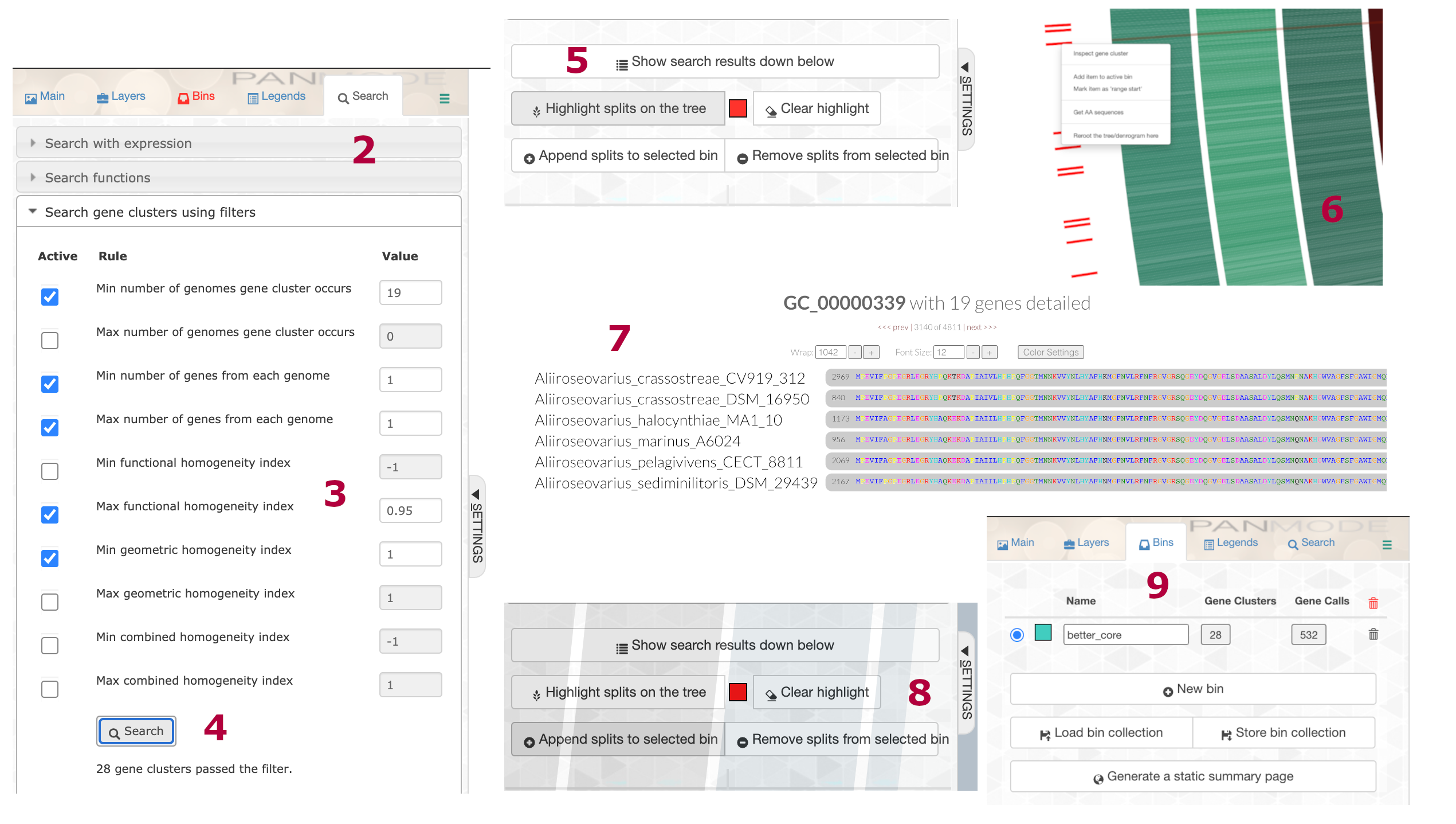
- Right click on a gene cluster and hit Inspect gene cluster.
- Check out the cluster, inspect others, make sure they look good.
- Head back to the button under Highlight and hit Append splits to the selected bin.
- Go to the Bins tab, rename the bin if you wish, and click Store bin collection.
We relaxed the functional homogeneity index to accommodate the outgroup. The pangenome database now has a new collection of SCG and a new phylogenomic tree. The new collection has 28 gene clusters and 532 genes. 532 divided by 19 (number of genomes) equals 28. Sweet.
Optional, on the fly tree generation.
If you wish, you can use the curated collection of gene clusters to generate a new tree right in the interface.
- Head over to the Layers tab and click Generate new phylogenetic tree.
- In the popup window make sure you like the settings and hit Generate.
Rather than using the tree generated on the fly by anvi’o, let’s get the sequences from the curated bin collection and do the analysis ourselves.
anvi-get-sequences-for-gene-clusters -p Aliiroseovarius-PAN.db \
                                     -g Aliiroseovarius-GENOMES.db \
                                     -C default -b better_core \
                                     --concatenate-gene-clusters \
                                     --align-with muscle \
                                     -o Aliiroseovarius-proteins-better-core.fa
Under this scenario, anvi’o retrieves, aligns (in this case with MUSCLE (Edgar 2004)), and then concatenates the sequences.
It is important to note that everything we just in the interface can instead be done in the command line. If you look at the help menu for anvi-get-sequences-for-gene-clusters you will see that you can apply the filtering steps described above directly in the command line without the pangenomic interactive. Personally, I like to use the interactive because I can visually inspect each gene cluster to make sure nothing fishy is going on. The parameters you choose will depend on your question and the peculiarities of your data set, so play around.
Just for the fun of it, let’s have a look at what this entails without running interactive.
anvi-get-sequences-for-gene-clusters -p Aliiroseovarius-PAN.db \
                                     -g Aliiroseovarius-GENOMES.db \
                                     -o Aliiroseovarius-proteins-better-core_no_interactive.fa
                                     --concatenate-gene-clusters \
                                     --min-num-genomes-gene-cluster-occurs 19  \
                                     --min-num-genes-from-each-genome 1 \
                                     --max-num-genes-from-each-genome 1 \
                                     --max-functional-homogeneity-index 0.95 \
                                     --min-geometric-homogeneity-index 1.00
And the last part of the output looks like this:
INFO
===============================================
Your filters resulted in 28 gene clusters that contain a total of 532 genes.
for downstream analyses. Just so you know.

Sequence type ...............................................: Amino acid
Output file for phylogenomics ...............................: Aliiroseovarius-proteins-better-core_no_interactive.fa
As expected, 28 gene clusters encompassing a total of 532 genes. Note, the order of genes in the concatenate file may differ but the content should be the same.
Anyway, regardless of the approach you choose, now we can use your curated SCG fasta file to construct a new phylogenomic tree. You can either do this is anvi’o, which will use IQ-TREE (Minh et al. 2020), or you can run a program outside anvi’o.
The anvi’o way…
anvi-gen-phylogenomic-tree -f Aliiroseovarius-proteins-better-core.fa \
                           -o Aliiroseovarius-proteins-better-core.tre
Generating & Visualizing Tree
Instead, we will use IQ-TREE (Minh et al. 2020) (v. 2.0.3) natively with ModelFinder Plus (Kalyaanamoorthy et al. 2017) to perform extended model selection followed by tree inference. ModelFinder computes the log-likelihoods of an initial parsimony tree for many different models then computes Akaike information criterion (AIC), corrected Akaike information criterion (AICc), and the Bayesian information criterion (BIC) to choose the substitution model that minimizes the BIC score.
iqtree -s Aliiroseovarius-proteins-better-core.fa \
                    --prefix aliiroseovariusMFP  \
                    -m MFP -T $NSLOTS
ModelFinder tested 48 models (it will test up to 546 protein models) and selected LG+F+I+G4 as the best-fit model based on BIC. We subsequently ran this model with 5000 ultrafast bootstrap approximations (Hoang et al. 2017).
iqtree -s Aliiroseovarius-proteins-better-core.fa \
       --prefix aliiroseovariusLG+F+I+G4-5000  \
       -m LG+F+I+G4 -bb 5000 -T $NSLOTS
Great, we have a tree but really no other information to decorate it with. So far, we have generated a lot of metric data for each genome. Luckily, all of that is in the pangenome database. We use the command anvi-export-misc-data to get most what we need.
anvi-export-misc-data --pan-or-profile-db Aliiroseovarius-PAN.db \
                      --target-data-table layers \
                      --output-file genome_stats.txt
This table contains things like total length, GC content, percent completion, percent redundancy, and so on. One piece we do not have by may want is the SCG taxonomy, specifically the genus prediction.
We did this way back in the beginning, but let’s do it again for our final collection.
for genome in `cat final_genomes.txt`
do
       anvi-estimate-scg-taxonomy \
        -c 03_CONTIGS/$genome-contigs.db \
        -o 09_SCG_TAXONOMY/$genome-SCG.txt
done
And add these data to our file with genome stats. Most of the lineage data is uninformative and can be eliminated. We also constructed a metadata file after sifting through all of the metadata we retrieved from NCBI about natural host and isolation source. We could combine these files but I like to keep the metadata file separate so I can add info as needed. Time to visualize.
Since we do not have a database, anvi’o will create a dummy database the first time we run the command anvi-interactive. But we still must give a name for the as yet nonexistent database.
anvi-interactive --profile-db profile.db
                 --tree aliiroseovariusLG+F+I+G4-5000.treefile
                 --manual
Stop the interactive. Now we have a database to populate. Let’s add the genome metric data.
anvi-import-misc-data genome_stats.txt
                 --pan-or-profile-db profile.db
                 --target-data-table items
Now we can restart the interactive with our metadata file of NCBI collection info.
anvi-interactive --profile-db profile.db
                 --tree aliiroseovariusLG+F+I+G4-5000.treefile
                 --additional-layers metadata.txt
                 --manual
If you are unfamiliar with IQ-TREE, check out the tutorial. It’s a really nice program.
Genome Metadata
Here is the metadata for record of all genomes used in phylogenomic analysis of MAG04. Table contains information for each of the 14 Aliiroseovarius (plus 4 outgroup genomes). Description of table headers are as follows.
genome_id: Name of genome in phylogenomic tree.
isolation_category: Broad category based on host/isolation source information retrieved from the BioSample record.
organism: Organism name retrieved from the BioSample record.
strain_or_isolate: Genome stain or isolate designation.
sample_information: Host/isolation source information retrieved from the BioSample record.
bioproject: NCBI BioProject ID.
biosample: NCBI BioSample ID.
assembly_accession: NCBI Assembly ID.
taxid: NCBI Taxonomy ID.
species_taxid: NCBI Species Taxonomy ID.
doi_publication: DOI link for related publication.
assembly_level: Assembly level.
seq_rel_date: Genome release data.
ftp_path: FTP link to download genome.
submitter: Submitting Institution.
A plain text version of this table (without HTML tags) can be downloaded here.
Conclusion
Dandy. Now we have a phylogenomic tree of MAG04 with 14 other Aliiroseovarius genomes and 4 from Roseovarius as the outgroup.
Source Code
The source code for this page can be accessed on GitHub by clicking this link.
Data Availability
Files generated from the pangenomic (01_MAG04_PAN/) and phylogenomic (02_MAG04_PHYLOGENOMICS) analyses of MAG04 can be downloaded from figshare at doi:10.25573/data.14774802. You can use the anvi’o commands described above to visualize the data.
In the analysis, this MAG is named WATER_MAG_00004. For brevity we refer to it henceforth as MAG04↩︎